Flow Charts
Context provides a charts module to create flow charts. The details are in the Charts uncovered manual by Pragma. There is also Flowchart creater to create flowchart code using javascript.
For example
\usemodule[chart]
\setupFLOWcharts[height=3\lineheight]

\startFLOWchart[example]
\startFLOWcell
  \name {flow}
  \location {1,1}
  \text {Flow}
  \connection [rl] {chart}
\stopFLOWcell
\startFLOWcell
  \name {chart}
  \location{2,1}
  \text {Charts}
\stopFLOWcell
\stopFLOWchart
\FLOWchart[example]

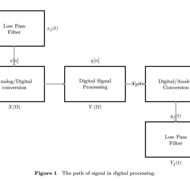
The more sophisticated example:
\usemodule[chart]

\setupFLOWcharts
[nx=5,
ny=3,
dx=2\bodyfontsize,
dy=2\bodyfontsize,
maxwidth=\textwidth
]

\setupFLOWshapes
[framecolor=black,
background=color,
backgroundcolor=white,
]

\startFLOWchart[DSP]

	\startFLOWcell
	\name{input}
	\location{1,1}
	\shape{44}
	\connection[rl] {lowpass1}
	\comment[t]{$x(t)$}
	\comment[b]{$X(t)$}
	\stopFLOWcell

	\startFLOWcell
	\name {lowpass1}
	\location {2,1}
	\text {Low Pass\crlf Filter}
	\connection[bt] {adconv}
	\comment[r]{$x_f(t)$}
	\comment[l]{$X_f(t)$}
	\stopFLOWcell

	\startFLOWcell
	\name{adconv}
	\location{2,2}
	\text{Analog/Digital\crlf conversion}
	\connection[rl]{dsp}
	\comment[t]{$x[n]$}
	\comment[b]{$X(\Omega)$}
	\stopFLOWcell

	\startFLOWcell
	\name{dsp}
	\location{3,2}
	\text{Digital Signal\crlf Processing}
	\connection[rl]{daconv}
	\comment[t]{$y[n]$}
	\comment[b]{$Y(\Omega)$}
	\stopFLOWcell

	\startFLOWcell
	\name{daconv}
	\location{4,2}
	\text{Digital/Analog\crlf Conversion}
	\connection[bt]{lowpass2}
	\comment[r]{$y_d(t)$}
	\comment[l]{$Y_d(t)$}
	\stopFLOWcell

	\startFLOWcell
	\name {lowpass2}
	\location {4,3}
	\text {Low Pass\crlf Filter}
	\connection[rl]{output}
	\comment[t]{$y_f(t)$}
	\comment[b]{$Y_f(t)$}
	\stopFLOWcell

	\startFLOWcell
	\name {output}
	\location {5,3}
	\shape{44}
	\stopFLOWcell

\stopFLOWchart

\placefigure[here][fig:chart]{The path of signal in digital processing.}
{
	\FLOWchart[DSP]
}