Difference between revisions of "Flow Charts"
Jump to navigation
Jump to search
m (added Category Graphics) |
m (fix typo) |
||
| (15 intermediate revisions by 7 users not shown) | |||
| Line 1: | Line 1: | ||
| − | + | Context provides a charts module to create flow charts. | |
| + | The details are in the [[manual:mchart.pdf|Charts uncovered]] manual by Pragma. | ||
| − | + | For example | |
| + | |||
| + | <context source="yes"> | ||
| + | \usemodule[chart] | ||
| + | \setupFLOWcharts[height=3\lineheight] | ||
| + | |||
| + | \startFLOWchart[example] | ||
| + | \startFLOWcell | ||
| + | \name {flow} | ||
| + | \location {1,1} | ||
| + | \text {Flow} | ||
| + | \connection [rl] {chart} | ||
| + | \stopFLOWcell | ||
| + | \startFLOWcell | ||
| + | \name {chart} | ||
| + | \location{2,1} | ||
| + | \text {Charts} | ||
| + | \stopFLOWcell | ||
| + | \stopFLOWchart | ||
| + | \FLOWchart[example] | ||
| + | </context> | ||
| + | |||
| + | The more sophisticated example: | ||
| + | |||
| + | <context source="yes"> | ||
| + | \usemodule[chart] | ||
| + | |||
| + | \setupFLOWcharts | ||
| + | [nx=5, | ||
| + | ny=3, | ||
| + | dx=2\bodyfontsize, | ||
| + | dy=2\bodyfontsize, | ||
| + | maxwidth=\textwidth | ||
| + | ] | ||
| + | |||
| + | \setupFLOWshapes | ||
| + | [framecolor=black, | ||
| + | background=color, | ||
| + | backgroundcolor=white, | ||
| + | ] | ||
| + | |||
| + | \startFLOWchart[DSP] | ||
| + | |||
| + | \startFLOWcell | ||
| + | \name{input} | ||
| + | \location{1,1} | ||
| + | \shape{44} | ||
| + | \connection[rl] {lowpass1} | ||
| + | \comment[t]{$x(t)$} | ||
| + | \comment[b]{$X(t)$} | ||
| + | \stopFLOWcell | ||
| + | |||
| + | \startFLOWcell | ||
| + | \name {lowpass1} | ||
| + | \location {2,1} | ||
| + | \text {Low Pass\crlf Filter} | ||
| + | \connection[bt] {adconv} | ||
| + | \comment[r]{$x_f(t)$} | ||
| + | \comment[l]{$X_f(t)$} | ||
| + | \stopFLOWcell | ||
| + | |||
| + | \startFLOWcell | ||
| + | \name{adconv} | ||
| + | \location{2,2} | ||
| + | \text{Analog/Digital\crlf conversion} | ||
| + | \connection[rl]{dsp} | ||
| + | \comment[t]{$x[n]$} | ||
| + | \comment[b]{$X(\Omega)$} | ||
| + | \stopFLOWcell | ||
| + | |||
| + | \startFLOWcell | ||
| + | \name{dsp} | ||
| + | \location{3,2} | ||
| + | \text{Digital Signal\crlf Processing} | ||
| + | \connection[rl]{daconv} | ||
| + | \comment[t]{$y[n]$} | ||
| + | \comment[b]{$Y(\Omega)$} | ||
| + | \stopFLOWcell | ||
| + | |||
| + | \startFLOWcell | ||
| + | \name{daconv} | ||
| + | \location{4,2} | ||
| + | \text{Digital/Analog\crlf Conversion} | ||
| + | \connection[bt]{lowpass2} | ||
| + | \comment[r]{$y_d(t)$} | ||
| + | \comment[l]{$Y_d(t)$} | ||
| + | \stopFLOWcell | ||
| + | |||
| + | \startFLOWcell | ||
| + | \name {lowpass2} | ||
| + | \location {4,3} | ||
| + | \text {Low Pass\crlf Filter} | ||
| + | \connection[rl]{output} | ||
| + | \comment[t]{$y_f(t)$} | ||
| + | \comment[b]{$Y_f(t)$} | ||
| + | \stopFLOWcell | ||
| + | |||
| + | \startFLOWcell | ||
| + | \name {output} | ||
| + | \location {5,3} | ||
| + | \shape{44} | ||
| + | \stopFLOWcell | ||
| + | |||
| + | \stopFLOWchart | ||
| + | |||
| + | \placefigure[here][fig:chart]{The path of signal in digital processing.} | ||
| + | { | ||
| + | \FLOWchart[DSP] | ||
| + | } | ||
| + | </context> | ||
| + | |||
| + | ==Syntax for {{cmd|connection}}== | ||
| + | |||
| + | <texcode> | ||
| + | \connection [<from><to>] {<FLOWcell>} | ||
| + | </texcode> | ||
| + | |||
| + | <code><from></code> and <code><to></code> are the points from which point to which point the connection should be drawn. The following graphic depicts the names of the points. | ||
| + | |||
| + | <texcode> | ||
| + | -t t +t | ||
| + | ---------------- | ||
| + | +l | | +r | ||
| + | | | | ||
| + | l | | r | ||
| + | | | | ||
| + | -l | | -r | ||
| + | | | | ||
| + | ---------------- | ||
| + | -b b +b | ||
| + | |||
| + | </texcode> | ||
| + | |||
| + | ===Example=== | ||
| + | |||
| + | The following code draws a line from the left top point of the current cell to the right bottom point of cell <code>foobar</code>. | ||
| + | |||
| + | <texcode> | ||
| + | \connection [-t+b] {foobar} | ||
| + | </texcode> | ||
| + | |||
| + | The code for connections in the pdf manual, e.g. | ||
| + | |||
| + | <texcode> | ||
| + | \connection[nb,pt]{episode_02_title} | ||
| + | </texcode> | ||
| + | No longer works | ||
| + | |||
| + | ==Aligning text within the cell== | ||
| + | |||
| + | To align left or right, use | ||
| + | |||
| + | <texcode> | ||
| + | \text[l]{left} | ||
| + | \text[r]{right} | ||
| + | </texcode> | ||
| + | |||
| + | Forcing a paragraph break with \par in a cell does not work... | ||
| + | |||
| + | <texcode> | ||
| + | \text[l]{firstline \par secondline} | ||
| + | </texcode> | ||
| + | |||
| + | Whereas using \\ does work, so: | ||
| + | |||
| + | <texcode> | ||
| + | \text[l]{firstline \\ secondline} | ||
| + | </texcode> | ||
| + | |||
| + | == Further hints == | ||
| + | |||
| + | * [[manual:mchart.pdf|Charts uncovered]] manual | ||
| + | * There was a [http://www.im.ps.pl/context/?en Flowchart creater] to create flowchart code using javascript, but it disappeared. | ||
| + | * The [[manual:nodes.pdf|nodes module]] covers even more applications of charts. | ||
[[Category:Graphics]] | [[Category:Graphics]] | ||
| + | [[Category:Metapost]] | ||
| + | [[Category:Sciences]] | ||
Latest revision as of 09:29, 1 July 2022
Context provides a charts module to create flow charts. The details are in the Charts uncovered manual by Pragma.
For example
\usemodule[chart]
\setupFLOWcharts[height=3\lineheight]

\startFLOWchart[example]
\startFLOWcell
  \name {flow}
  \location {1,1}
  \text {Flow}
  \connection [rl] {chart}
\stopFLOWcell
\startFLOWcell
  \name {chart}
  \location{2,1}
  \text {Charts}
\stopFLOWcell
\stopFLOWchart
\FLOWchart[example]

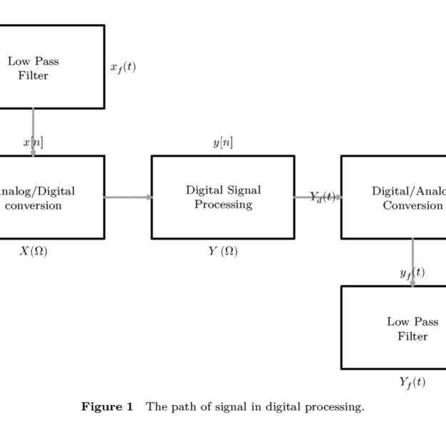
The more sophisticated example:
\usemodule[chart]

\setupFLOWcharts
[nx=5,
ny=3,
dx=2\bodyfontsize,
dy=2\bodyfontsize,
maxwidth=\textwidth
]

\setupFLOWshapes
[framecolor=black,
background=color,
backgroundcolor=white,
]

\startFLOWchart[DSP]

	\startFLOWcell
	\name{input}
	\location{1,1}
	\shape{44}
	\connection[rl] {lowpass1}
	\comment[t]{$x(t)$}
	\comment[b]{$X(t)$}
	\stopFLOWcell

	\startFLOWcell
	\name {lowpass1}
	\location {2,1}
	\text {Low Pass\crlf Filter}
	\connection[bt] {adconv}
	\comment[r]{$x_f(t)$}
	\comment[l]{$X_f(t)$}
	\stopFLOWcell

	\startFLOWcell
	\name{adconv}
	\location{2,2}
	\text{Analog/Digital\crlf conversion}
	\connection[rl]{dsp}
	\comment[t]{$x[n]$}
	\comment[b]{$X(\Omega)$}
	\stopFLOWcell

	\startFLOWcell
	\name{dsp}
	\location{3,2}
	\text{Digital Signal\crlf Processing}
	\connection[rl]{daconv}
	\comment[t]{$y[n]$}
	\comment[b]{$Y(\Omega)$}
	\stopFLOWcell

	\startFLOWcell
	\name{daconv}
	\location{4,2}
	\text{Digital/Analog\crlf Conversion}
	\connection[bt]{lowpass2}
	\comment[r]{$y_d(t)$}
	\comment[l]{$Y_d(t)$}
	\stopFLOWcell

	\startFLOWcell
	\name {lowpass2}
	\location {4,3}
	\text {Low Pass\crlf Filter}
	\connection[rl]{output}
	\comment[t]{$y_f(t)$}
	\comment[b]{$Y_f(t)$}
	\stopFLOWcell

	\startFLOWcell
	\name {output}
	\location {5,3}
	\shape{44}
	\stopFLOWcell

\stopFLOWchart

\placefigure[here][fig:chart]{The path of signal in digital processing.}
{
	\FLOWchart[DSP]
}
Syntax for \connection
\connection [<from><to>] {<FLOWcell>}
<from> and <to> are the points from which point to which point the connection should be drawn. The following graphic depicts the names of the points.
       -t    t    +t
     ----------------
 +l |                | +r
    |                |
  l |                |  r
    |                |
 -l |                | -r
    |                |
     ----------------
       -b    b    +b
Example
The following code draws a line from the left top point of the current cell to the right bottom point of cell foobar.
\connection [-t+b] {foobar}
The code for connections in the pdf manual, e.g.
\connection[nb,pt]{episode_02_title}
No longer works
Aligning text within the cell
To align left or right, use
\text[l]{left}
\text[r]{right}
Forcing a paragraph break with \par in a cell does not work...
\text[l]{firstline \par secondline}
Whereas using \\ does work, so:
\text[l]{firstline \\ secondline}
Further hints
- Charts uncovered manual
- There was a Flowchart creater to create flowchart code using javascript, but it disappeared.
- The nodes module covers even more applications of charts.